Pages

Showing posts with label excel. Show all posts

Wednesday, March 28, 2012

Active x Data connection for MS SqlServer

Sub SQLServerDBAutomation()

    Dim cnct As New ADODB.Connection

    Dim recordset As New ADODB.recordset

    Dim col As Integer

    Cells.Clear

    'Open the connection

    cnct.Open "Provider=SQLOLEDB.1;Integrated Security=SSPI;Persist Security Info=True;Initial   Catalog=Facility ServicessSQL;Data Source=.\sqlexpress;Use Procedure for Prepare=1;Auto Translate=True;Packet _     Size=4096;Workstation ID=RAVI-PC;Use Encryption for Data=False;Tag with column collation when possible=False;"

    'Create RecordSet

    recordset.Open "select * from Employee_Master", cnct, adOpenKeyset

    'Write the field names

    For col = 0 To recordset.Fields.Count - 1

        Range("A1").Offset(0, col).Value = recordset.Fields(col).Name

    Next

    'Write the recordset

    If recordset.RecordCount > 0 Then

        Range("a1").Offset(1, 0).CopyFromRecordset recordset, recordset.RecordCount, recordset.Fields.Count

    End If

    Set recordset = Nothing

    Set cnct = Nothing

End Sub

MS Access ADODB Connection

Sub AccessDBAutomation()
    Dim cnct As New ADODB.Connection
    Dim recordset As New ADODB.recordset
    Dim col As Integer
    Cells.Clear
    'Open the connection
    cnct.Open "Provider=Microsoft.ACE.OLEDB.12.0;User ID=Admin;Data Source=C:\Users\Ravi\Desktop\budget data.accdb;"
    'Create RecordSet
    recordset.Open "SELECT * FROM Budget", cnct, adOpenKeyset
    'Write the field names
    For col = 0 To recordset.Fields.Count - 1
        Range("A1").Offset(0, col).Value = recordset.Fields(col).Name
    Next
    'Write the recordset
    If recordset.RecordCount > 0 Then
        Range("a1").Offset(1, 0).CopyFromRecordset recordset, recordset.RecordCount, recordset.Fields.Count
    End If
    Set recordset = Nothing
    Set cnct = Nothing
End Sub

Wednesday, December 14, 2011

New Features in Excel 2010 Conditional Formatting


Excel 2010 - Conditional Formatting - Review, Improvements and Demo
Conditional formatting is one of favorite features in Excel. CF has helped me save the day at work more than a dozen occasions. I almost became project manager just because I knew how to make a gantt chart in excel using conditional formatting. I have written extensively about it.
So, I was naturally curious to explore what is new in Excel 2010′s Conditional Formatting. In this post, I will share some of the coolest improvements in CF.

1. You can refer to data in other worksheets now

Refer values in other worksheets - excel conditional formatting
This is the best new addition to CF capabilities in Excel 2010. Now we can refer to data in other worksheets without using any named ranges or copying the data over to primary sheet.

2. Solid Data Bars, Finally!

In Excel 2007, MS introduced a new feature called “data bars”. It felt like an exciting thing, except for one gnawing problem. The bars have gradients. So, not only they looked ugly, but they were also difficult to read (also, they were inaccurate at default settings).
Thankfully MS rectified these problems and significantly improved data bars in Excel 2010.
Now, you can,
  • Create data bars with solid fill
  • Apply borders to data bars (so that even gradient fills look elegant)
  • Have negative data bars
  • Have an axis so that comparison is easy
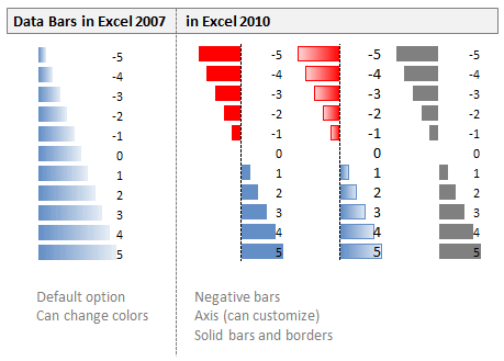
Here is a small comparison between Excel 2007 & Excel 2010 Data Bars:
Data Bars in Excel 2007 vs. Excel 2010 - a comparison

Using data bars to create in-cell progress charts:

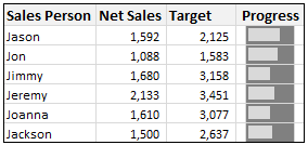
You can use data bars to create in-cell progress charts (or thermo-meter charts) like this:
An In-cell Progress Chart - Excel Conditional Formatting Trick
* Hint: The trick is to use cell background color along with data bar.
[Related: Jon Peltier has written a beautiful article reviewing data bars in Excel 2010.]

3. More Icon Sets in Conditional Formatting

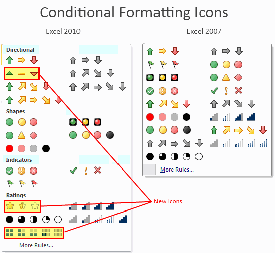
Although I rarely use icons in conditional formatting, I am happy to report that MS has added 3 new sets of Icons to the conditional formatting library.
Icon Sets in Excel 2010 Conditional Formatting - Compared with Excel 2007
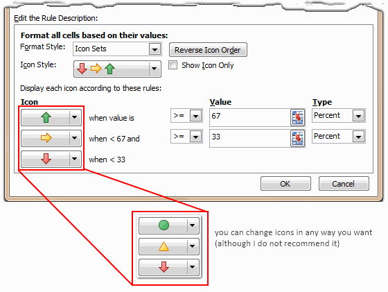
Also, you can mix and match icons depending on the rules (how I wish they didnt allow this. Mix and match can produce more evil combinations than good ones.)
Mix and Match Icons in Excel 2010 CF - Use with care

Tuesday, December 13, 2011

compare 2 lists


Even Faster Way to Compare 2 Lists in Excel [Quick Tip]


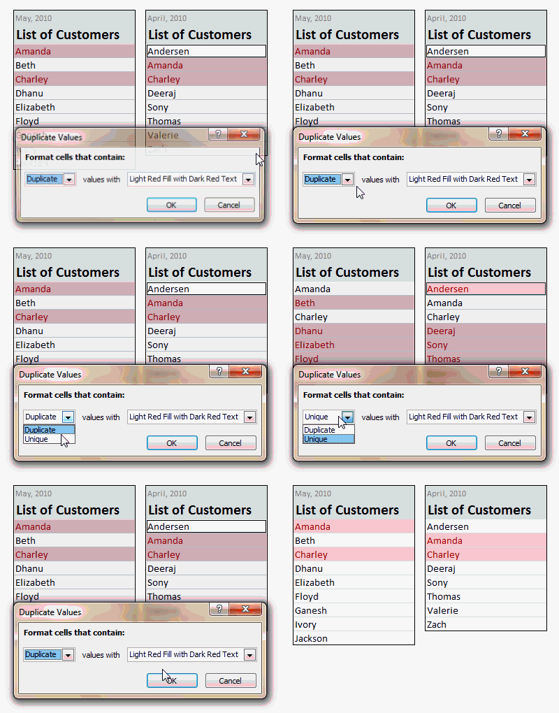
The quickest way to find all about two lists is to select them both and them click on Conditional Formatting -> Highlight cells rules -> Duplicate Values (Excel 2007). The result is that it highlights in both lists the values that ARE the same. Then in one list non-highlighted are values that are not present in the second list, and opposite for the second list. I think it is sell “geeky”, but it gets job done very very quickly when you don’t want to mess around.

A Ridiculously easy and fun way to compare 2 lists

Compare 2 lists of Data in Excel - Conditional Formatting Tip[works only Excel 2007+, use theabove technique if you are on excel 2003 or earlier]
  1. Select cells in both lists (select first list, then hold CTRL key and then select the second)
  2. Go to Conditional Formatting > Highlight Cells Rules > Duplicate Values
  3. Press ok.
  4. There is nothing do here. Go out and play!
See the screencast aside to see how this works

Sunday, December 11, 2011

How to Outline an Excel Worksheet

What’s new in Excel 2010?


Here’s a quick overview of the new features in Excel 2010:
● 64-bit version: If your hardware and Windows version supports it, you can install the 64-bit
version, which lets you create larger workbooks. You might experience some incompatible
macros and add-ins. Specifically, macros that use 32-bit Windows API calls won’t work in
64-bit Excel 2010. In most cases, however, you can modify the code so that the API calls
work with both versions of Excel.
● Sparkline charts: Create small in-cell charts to summarize a range of data graphically.
● Slicers: A slicer is a new way to filter and display data in pivot tables.
● New pivot table formatting options: You have more control over the appearance of pivot
table reports.
● Office button changes: The big round Office button in Excel 2007 has been replaced by a
File button, displayed to the left of the tabs. Clicking it displays Office Backstage, a screen
that lets you perform various operations on your workbook. This view essentially replaces
the traditional File and Print menus — plus quite a bit more.
● Conditional formatting enhancements: Data bar conditional formatting can display in a
solid color, and the bars provide a more accurate display and support negative values.
● Function enhancements: Some of Excel’s worksheet financial and statistical functions
have been improved in terms of numerical accuracy. These functions have new names, and
the old versions are still available for compatibility.
● Image-editing enhancements: You have much more control over graphic images inserted
into a workbook, including the ability to remove non-essential parts from the background
of an image.
● Screen capture tool: You can easily capture a window from a different program and insert
the image on a worksheet.
● Paste preview: When you copy a range, the Paste command displays various options with
a live preview so that you can see how the paste operation will look.
● Ribbon customization: End users can customize the Ribbon by adding new tabs and
groups. Unfortunately, it’s still not possible to customize the Ribbon using VBA.
● Equation editor: You can create and display (noncalculating) mathematical equations and
embed them on a worksheet.
● Faster: Microsoft made some improvements to the calculation engine, and files load a bit faster.
● New security features: Workbooks downloaded from the Internet or from e-mail attachments
are opened in Protected View mode. You can designate workbooks as trusted, and
they don’t need to reside in special trusted folders.
● Solver: Excel 2010 includes a new version of the Solver add-in.
● Enhancements to VBA: You can now perform operations that used to require old XLM
macros directly using VBA macro commands. In addition, macro recording now works for
operations such as chart and shape formatting.

Insert Picture Into Comment

Table Schmable, I Want Results!

No Duplicates Allowed In Row, Data Validation Custom Logic Formula COUNTIF

Rounding Invoices

Labels from Excel Data to Word 2010

Picture Lookup

Merge Tables with Copy, Paste and Clipboard

Clear Contents Of Worksheet Keep Formatting & Formulas & Other Clear

Drill Through Conditional Formatting Across Sheets Using Format Painter

Sunday, December 4, 2011


‎15 GREAT THOUGHTS BY CHANAKYA

1) "Learn from the mistakes of others... you can't live long enough to make them all yourselves!!"


2)"A person should not be too honest. Straight trees are cut first and Honest people are screwed first."


3)"Even if a snake is not poisonous, it should pretend to be venomous."


4)"There is some self-interest behind every friendship. There is no friendship without self-interests. This is a bitter truth."


5)" Before you start some work, always ask yourself three questions - Why am I doing it, What the results might be and Will I be successful. Only when you think deeply and find satisfactory answers to these questions, go ahead."


6)"As soon as the fear approaches near, attack and destroy it."


7)"The world's biggest power is the youth and beauty of a woman."


8)"Once you start a working on something, don't be afraid of failure and don't abandon it. People who work sincerely are the happiest."


9)"The fragrance of flowers spreads only in the direction of the wind. But the goodness of a person spreads in all direction."


10)"God is not present in idols. Your feelings are your god. The soul is your temple."


11) "A man is great by deeds, not by birth."


12) "Never make friends with people who are above or below you in status. Such friendships will never give you any happiness."


13) "Treat your kid like a darling for the first five years. For the next five years, scold them. By the time they turn sixteen, treat them like a friend. Your grown up children are your best friends."


14) "Books are as useful to a stupid person as a mirror is useful to a blind person."


15) "Education is the Best Friend. An Educated Person is Respected Everywhere. Education beats the Beauty and the Youth."
.
.
.
.
If you Like it Share with your Friends

Thursday, December 1, 2011

The Excel part of mail merge


Hey, the holidays are fast approaching, which means you've got to get your cards signed, sealed, and delivered! This post goes out to those of you who keep your address list in Excel and need to figure out how to use it to create mailing labels in Word.
Creating labels can be intimidating, mainly because there are a number of intricate steps to follow and you're typically working with different programs—in this case, Excel and Word. And if you create labels infrequently, it's hard to remember what to do and what to watch out for.
Learning how to make your Excel address list magically show up on your sheets of labels boils down to five basic steps:
Overview of five-step process for creating labels
This post is about that first step—the one where you prepare your address list in Excel so that you can use it in Word. If you get this part of the process right, things will run more smoothly when you're setting up your labels in Word.

Preparing your addresses in Excel

The key thing to understand is that your column headers, or categories, in Excel will become merge fields(placeholders) in Word. Each merge field corresponds to a piece of the address on the label—first name, last name, street address, and so on. Word pulls out the information in your Excel columns and plugs it into the corresponding merge fields, with an end result that looks something like this:
Data from Excel columns appearing on label
When setting up your address list in Excel, consider the following tips:
  • Use "friendly" column headers such as First Name, Last Name, Address, and City instead of Column 1, Column 2, Column 3, and Column 4.
  • Set up your address list so that each column represents the smallest possible piece of information. For example, use separate columns for First Name and Last Name rather than just a Name column. This practice gives you more flexibility if you end up creating cards or letters in addition to labels.
  • Avoid blank rows and columns in your address list. During the mail merge, these blanks can trick Word into thinking that it has reached the end of the address list, when in fact there is more information after the blanks.
  • To make it easier to pick the address list you want Word to use, give it an easily recognized name in Excel. To do this, select the range of cells that make up your address list. Then, in the Name box next to the formula bar, type a name like Holiday_Cards and click OK.
  • Postal codes can be tricky. If you have a column containing postal codes, make sure you format that column as Text. Otherwise, Excel will strip out any zeros from the front of the postal code. If you're creating a new address list from scratch, be sure to format your column as text before you type the postal codes. If you're importing addreses into Excel from a .txt file, use the Text Import Wizard to format the appropriate columns as Text (as opposed to leaving them in the General format or in another number format that might mess up the mail merge).
By the way, if you want to create labels from your Outlook contacts, you can do that without first importing the contacts into Excel. Word can access your contacts directly from Outlook during the mail merge process. For the details, download this Mail Merge Made Easy guide. It will tell you exactly what to do, based on where you keep your contacts (Excel, Outlook, or another email program) and where you plan to print your labels (Word or Publisher).

Now, on to Word

Once everything is set up in Excel, you'll need to open Word and start your mail merge (Mailings tab | Start Mail Merge group | Start Mail Merge). The following articles do a good job of walking you through that process.

Now where on the network did I save my workbook?


I ask myself that question a lot, especially since I typically save my workbooks to SharePoint team sites on our corporate servers. If you, too, save and share files on your network, you can make your life easier by adding the Document Location box to the Quick Access Toolbar. 
Document Location box on Quick Access Toolbar
The Document Location box shows you exactly where your file is saved. If you need your coworkers to review or edit your workbook, just paste the link from this box into an email message and send it to them. Trust me—sending a link is way better than sending a file attachment!
Here's how to add this box to the ribbon:
  1. Click the arrow next to the Quick Access Toolbar, and then click More Commands. 

    Arrow that opens shortcut menu
     
  2. In the Excel Options dialog box, in the Choose commands from box, click Commands Not in the Ribbon.
     
  3. Scroll down to the Document Location command and double-click it to add it to the Quick Access Toolbar.

    Document Location command in Excel Options dialog box
     
  4. Click OK. At this point, you should see the Document Location box on your Quick Access Toolbar. (If you ever want to get rid of it, right-click the border of the box, and then click Remove from Quick Access Toolbar.)
This procedure applies to Excel 2010, but it works pretty much the same way in Excel 2007. To quickly open theExcel Options dialog box in Excel 2010 or earlier, press ALT, and then press T, O.