Pivot Table Tricks to Make You a Star

We, data junkies, love pivot tables. We think pivot tables are solution for everything (except for may be global warming and that broken espresso machine down stairs).

Today, we are going to learn 5 awesome pivot table tricks that will make you a star.

1. Drill down on your Pivots with Double click

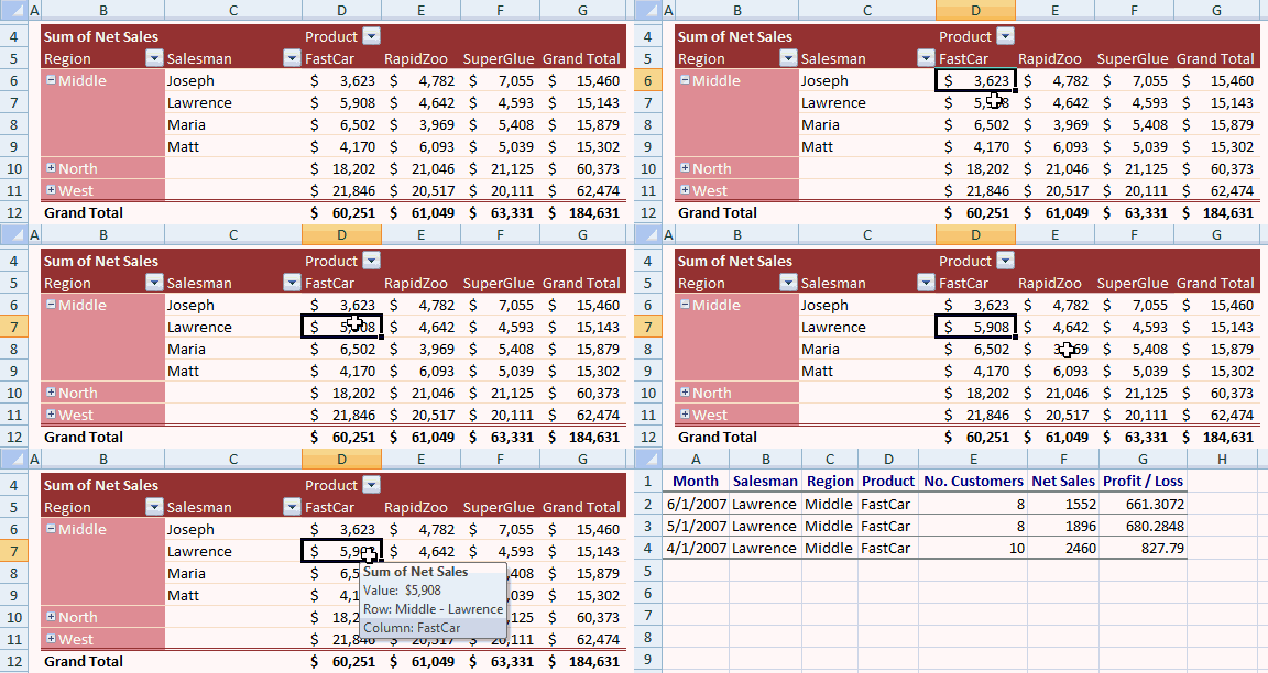
This is by far the simplest and most powerful pivot table trick I have learned. Whenever you want to see the values behind a pivot field just double click on it.

Lets say, the sales of Lawrence in Middle region  is $5,908 and you want to know which items contribute for this total, when you double click on the number $5,908 excel will show a list of all the records that add up to this number, neatly arranged in a new worksheet. Instant drill down.

See this magical trick in action.

2. Summarize Pivot Data by “Average” or some other formula

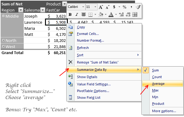
By default excel summarizes pivot data by “sum” or “count” depending on data type. But often you may want to change this to say “average”, to answer questions like “what is the average sales per product”. To do this, just right click on pivot table values (not on row or column headings) and select “summarize data by” and select “Average” option.

(In excel 2003, you have to do this from “field settings” menu option)

3. Slice & Dice your Pivot Tables with Grace

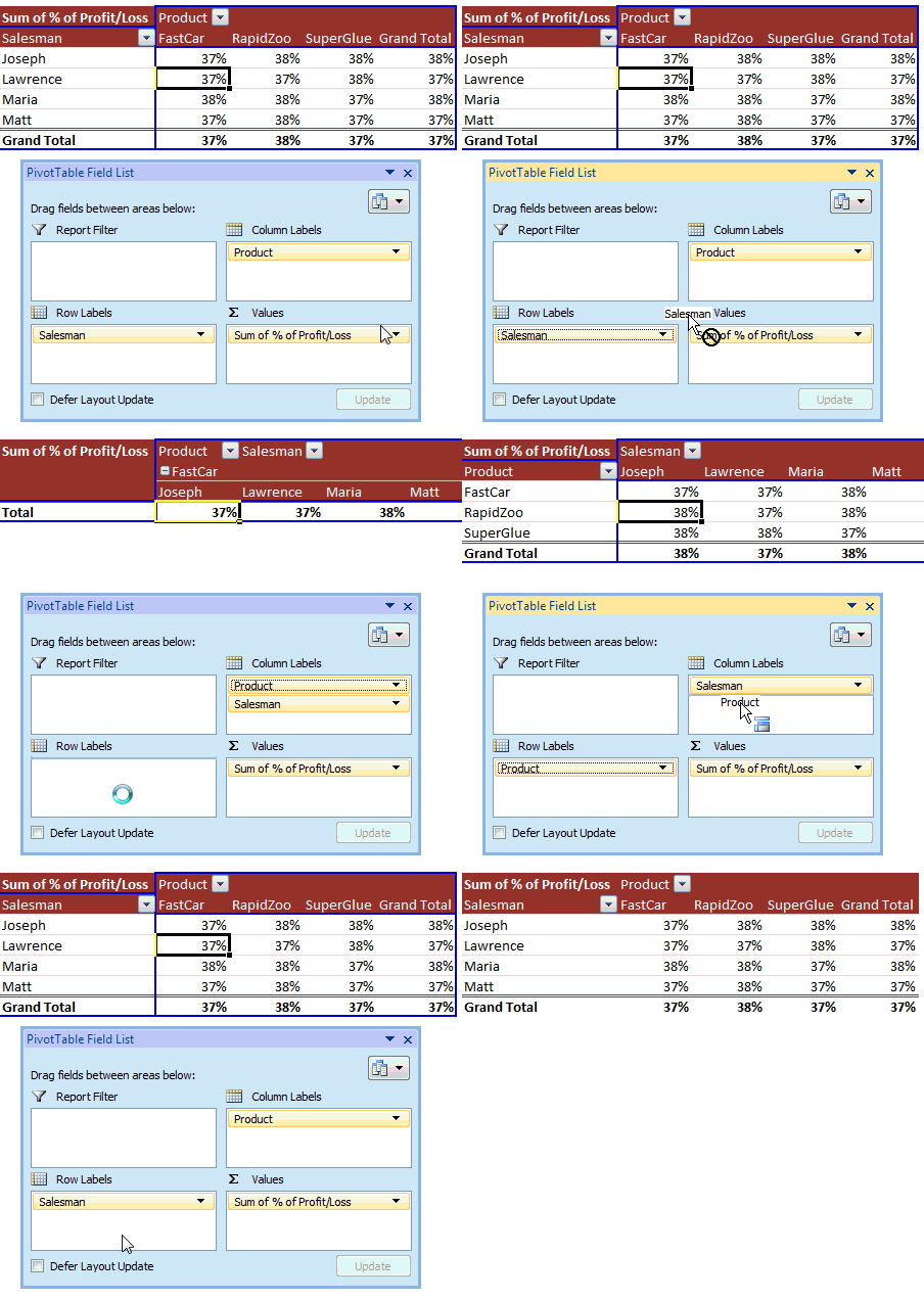
Re-arranging pivot table layouts is as easy as shuffling a pack of cards. Just drag and drop the fields from row areas to column areas (vice-a-versa) and you have the pivot table rearranged.

Here is a simple screencast explaining the secret

4. Show difference from last month (or year) without bending backwards

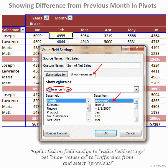
We all know that you can show monthly summaries using Pivots. But what if your boss wants you to also include “difference from previous month”  as well? Now, dont rush back to source data and add new columns. Here is the right trick to make you a star.

• Just use field settings to tell excel how you want the data to be summarized.
• Right click on any pivot table value, select “value field settings”
• Now go to “Show value as tab” and Change “Normal” to “Difference from”
• Select “Previous” from Base-item area. Leave Base field as-is.

Now, your pivot is updated to show difference from previous column.

Bonus: There are quite a few value field settings you can mess with. Go play and discover something fun. 

5. Add new dimensions to your Pivot Reports with Calculated Fields

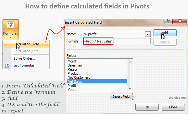
Let us say you have both “sale” and “profit” values in your source data. Now, your boss wants to know “profit %” in the pivot report (defined as Profit/Sales). You need not add any extra columns in your source data, instead you can define custom calculated fields with ease and use them in pivot reports.

• To do this, Go to pivot table options ribbon, select “formulas” > “calculated field”
• Now define a new calculated field by giving it a name and some meaningful formula.
• Make sure you adjust the cell formatting so that output of calculation can be displayed (for eg. change number to % format)

(In excel 2003, the formula option is available from Pivot menu in toolbar)

See this tip in action: